ELEC2311 - Lecture 6

← Back to Home

ELEC2311 - Lecture 5
VHDL Delay Models & Simulation Cycles - Slides

VHDL Delay Types

Real circuits have propagation delay and may suppress very short pulses. VHDL provides delay mechanisms to model these timing effects during simulation.

The two signal-assignment delay mechanisms are:

• Transport — prescribes propagation delay only
• Inertial — prescribes propagation delay and minimum input pulse width

Delay Signal Assignments are not Synthesisable

Transport Delay

Transport delay delays every signal change by a specified amount. Every pulse is propagated to the output, regardless of its duration.

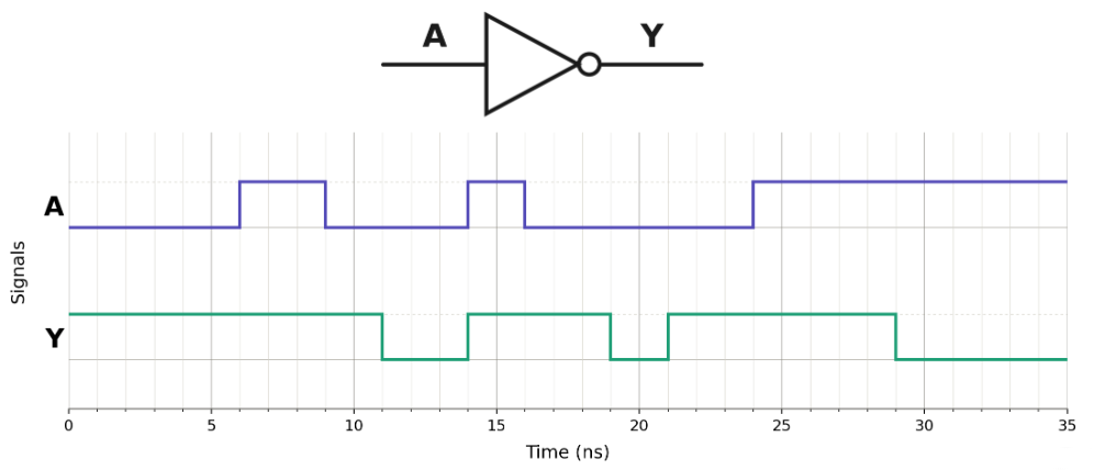
target <= transport expression after delay_time; 

Observe the effects of transport delay of an inverter:

Y <= transport not A after 5 ns;

The output is an exact match of the inverted input delayed by 5 ns.

Inertial Delay

Inertial delay models the behaviour of real-world devices that require a minimum input pulse width to register a change.

Inertial delay is the default delay type for signal assignment statements containing the after keyword.

target <= expression after delay_time; -- default inertial
-- or 
target <= inertial expression after delay_time; -- explicit
-- or 
target <= reject pulse_rejection_limit inertial expression after delay_time; 
-- pulse_rejection_limit must be between 0 ns and delay_time, inclusive 

The optional reject keyword specifies a pulse-rejection limit , which controls the filtering of short input pulses. If a pulse does not meet this limit, it isn’t transmitted to the output.

If reject isn’t specified, the pulse-rejection limit defaults to the specified inertial delay. The limit must be less than or equal to the inertial delay.

Given the example inverter with inertial delay defined by:

Y <= reject 2 ns inertial not A after 5 ns;

As seen on the graph, the 2 ns pulse does not pass through to the output.

---

Delta Cycle

Delta cycles $\Delta$ (also known as delta delay) are infinitely small, zero-time simulation steps used to evaluate concurrent events without advancing physical simulation time.

A delta cycle is split into two phases. The evaluate phase is where simulator checks active signals and runs processes sensitive to those changes. The update phase is where new signal values are assigned and scheduled.

Several delta cycles may occur at the same simulation time and time only moves forward once all delta cycles have been completed.

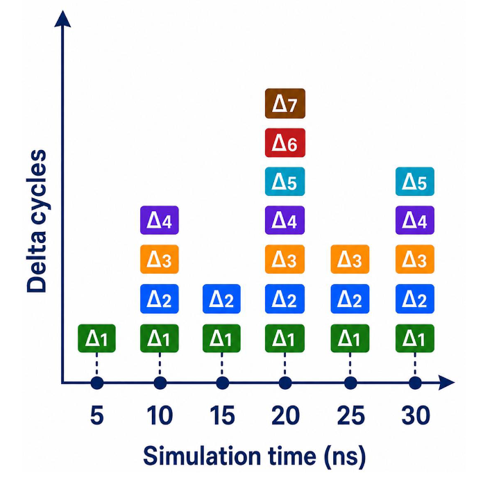
Delta cycles allow zero-delay signal changes to propagate between concurrent VHDL processes in a deterministic manner.

---

Transactions & Events

When the signal assignment Y <= X; is executed, the current value of X is evaluated and a transaction is scheduled for Y.

A transaction is a value-time pair specifying the value to be applied to a signal and the time at which it will be applied.

Every signal assignment schedules a transaction, but not every transaction produces an event.

When a scheduled transaction is applied, an event only occurs if the signal value changes. A signal may already have the scheduled value.

Variable Assignment

Variables are updated immediately when the assignment statement is executed. Unlike signal assignments, variable assignments do not schedule a transaction or involve a delta cycle.

Transaction Queue

When a transaction is created, it is inserted into the target signal’s queue in order of its scheduled times.

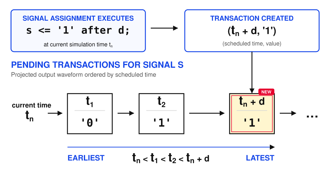
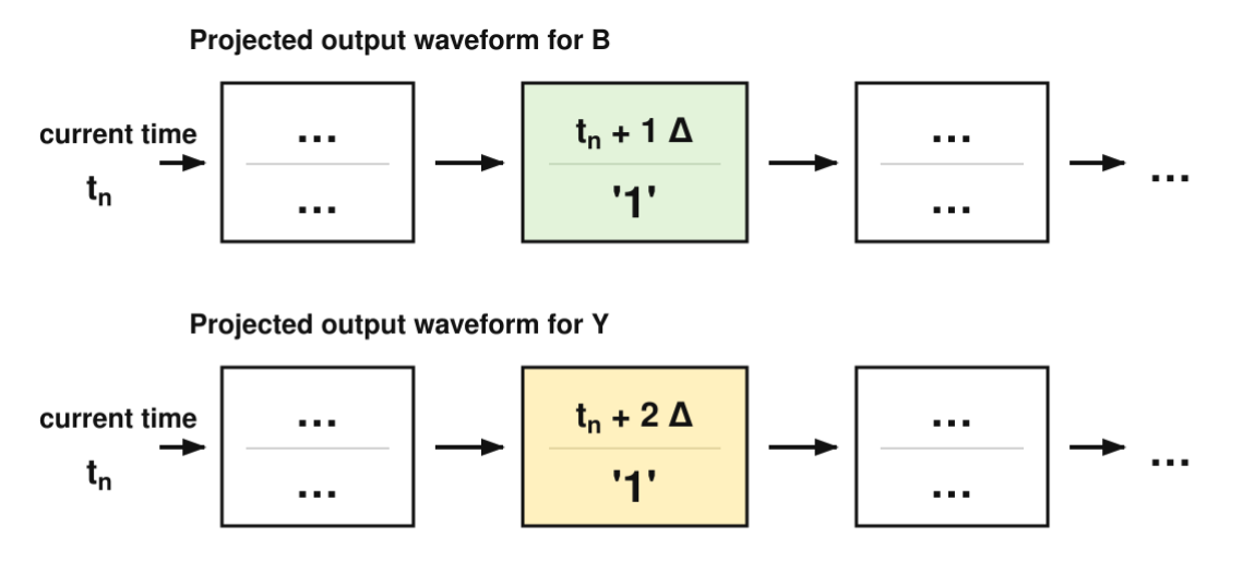
For a zero-delay assignment, (e.g. B <= A; Y <= B), the signal is not updated immediately. It is updated in a subsequent delta cycle $\Delta$ at the same simulation time.

Transaction Handling

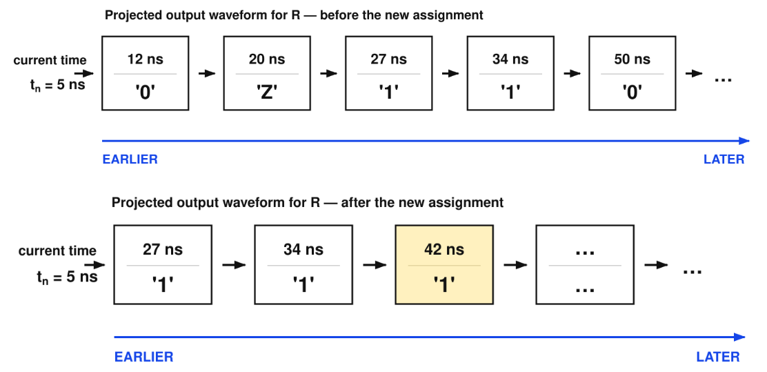
For a transport-delay assignment, all old transactions scheduled at or after the first new transaction time are removed.

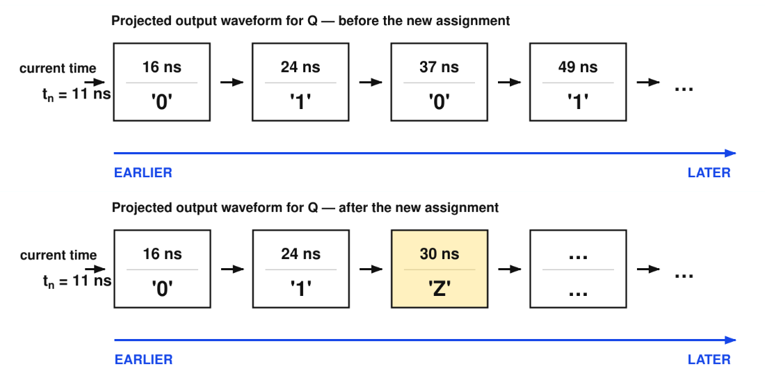
For an inertial-delay assignment, all old transactions scheduled at or after the first new transaction time are removed (like transport-delay).

Additionally, every transaction with a different value before the delay is removed if they have a time gap shorter than the inertial delay.

---

VHDL Simulation

Simulation Time

During simulation, a simulator keeps track of the current time that has been simulated. It is a representation of the circuit time, not the time the simulation has actually taken.

It is measured as an integral multiple of a basic unit of time known as the resolution limit. The simulator cannot measure time delays less than the resolution limit.

Simulation

Simulation alternates between two modes, event processing and statement execution.

Event processing is where transactions are applied. Statement execution is where resumed processes execute and future transactions are scheduled.

Initialisation Phase

The initialisation phase occurs at the very start of simulation.

1. Each signal is assigned an initial value, usually specified in the signal declaration. Simulation time is set to 0 and all processes are scheduled to execute.

2. When all processes have suspended, the initialisation phase ends. The simulation time is still set at 0. There should be a set of transactions scheduled to occur after this phase ends.

3. After the initialisation phase, the simulator then enters the main simulation loop. Each iteration of this loop is called a simulator cycle.

Simulation Cycle

The simulation cycle is the main simulation loop that governs the execution of the simulation. The cycle repeats until there are no further active signal drivers and no scheduled processes scheduled.

There are several steps in the simulation cycle:

1. Advance Time & Update Signals ($T_c\leftarrow T_n$)
   • Set current simulation time to next scheduled event time
   • Update all active signals with their new values
2. Trigger & Resume Processes
   • Mark triggered and pre-scheduled processes to run
3. Execute Active Processes
4. Schedule Next Event ($T_n$)
   • Occurs the next time a signal is active or process resumes

If $T_c=T_n$, the next simulation cycle is called a delta cycle, meaning the next event is to be processed at the current simulation time.

---

ELEC2311 - Lecture 7