CITS3011 - Lecture 3

← Back to Home

CITS3011 - Lecture 2
Informed Search - Slides

Uninformed vs Informed Search

Uninformed search selects nodes for expansion on the basis of distance/cost from the start state. There is no indication of how much distance is to go.

Informed search selects nodes for expansion using an estimate of distance to the goal state known as a heuristic. Requires additional information outside of the graph, but in exchange can find more efficient paths to goal.

---

Heuristic Function

A heuristic function is an estimate of how close a given state is to a goal. It is specific for any particular search problem.
$h(n)=\text{estimated cost from n to goal}$

$h(n)$ is also known as forward cost.

Manhattan Distances

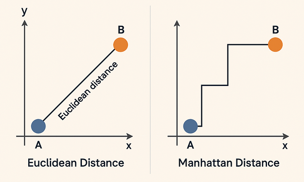
Manhattan distance is a metric that measures the distance between two points by summing the absolute differences between their coordinates.

Distance is calculated by moving only horizontally and vertically.

Admissible vs Consistent Heuristics

Admissible: $h(n)\le h^{\ast }(n)$ where $h^{\ast }(n)$ is actual cost from $n$ to goal -> $h(n)$ never overestimates for all $n$.

Consistent (monotonic): $h(n)\le c(n,a,n^{\prime })+h(n^{\prime })$, where $n’$ is a successor to $n$ by action $a$ -> estimated cost between nodes never decreases by more than actual step cost between them.

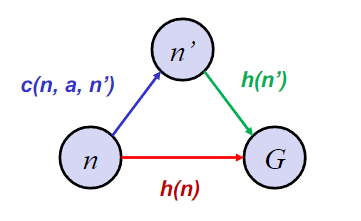
Every consistent heuristic is admissible, but not vice versa

Dominant Heuristics

A heuristic $h_2$ dominates a heuristic $h_1$ if, for every state $n$:

$h_2(n)\ge h_1(n)$

• Provided both heuristic are admissible.

$h_2$ is a strictly better heuristic than $h_1$.

---

Greedy Search

Greedy search is an informed search function that expands the node that appears to be closest to the goal. Nodes are ordered by their forward cost $h(n)$.

Is efficient, but not optimal: aims to explore the least amount of nodes and returns the first solution found.

Time Complexity	Space Complexity
$O(b^m)$	$O(b^m)$
Additionally, in infinite state spaces, a greedy function can be incomplete, looping forever between nodes with low forward cost connections.

Uniform Cost Search

Uniform cost search (UCS) is an uninformed search function that always expands the lowest-cost node next in a weighted graph. It uses a priority queue.

If it encounters a node it has already discovered and the new path to it is cheaper, it updates it with the lower cost in the queue.

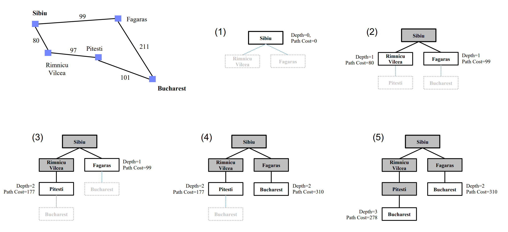
The goal node is only checked when it is popped from the queue, which ensures that the cheapest path to the goal is found. Thus, UCS is complete and optimal (as long as all step-costs $\ge 0$).

UCS has the trade-off of being expensive:

Time Complexity	Space Complexity
$O(b^{1+[C^{\ast }/ϵ]})$	$O(b^{1+[C^{\ast }/ϵ]})$
$[C^{\ast }/ϵ]$ is the maximum amount of steps and $b$ is the branching factor. Alternatively, the time/space complexity can be described as $n$, where $n$ is the number of tree nodes with cost less than optimum.

Link to original

---

A* Search

A* search expands nodes using an estimate of total path-cost $f(n)=g(n)+h(n)$. $g(n)$ is the actual cost from start to $n$ and $h(n)$ is the heuristic function.

Time Complexity	Space Complexity
$O(x)$	$O(x)$
A* search is both complete (unless $x=\infty$) and fairly efficient. It balances backwards cost (UCS) and forward estimate (Greedy). However, its optimality depends on the quality of its heuristic function.

A* Optimality

A* search can be done as a graph or tree search. Graph search uses a closed set to avoid repeated states and improves efficiency at the potential cost of optimality.

Search Type	Optimal if…
A* Tree Search	heuristic is admissible
A* Graph Search	heuristic is consistent

Variants of A*

Variant	Focus	Idea	Trade-Off
Weighted A*	Processing speed	$g(n)+\text{W}{}^{\ast }h(n)$	No longer guaranteed optimal path.
Anytime A*	Time-limited results	Start with large $\text{W}$, that shrinks over time.	Demands variable execution time to reach optimal solution.
Beam Search	More efficient	Limit search to only the top $k$-nodes.	Incomplete and suboptimal.
Iterative Deepening A* (IDA*)	Zero-queue memory	Modified DFS with cut-off at $f(n)$.	Re-explores nodes repeatedly.
Simplified Memory-Bounded A* (SMA*)	Maximum memory cap	Drops highest cost nodes from memory.	Needs to regenerate nodes if alternate paths fail.

---

Deriving Heuristics

There are two general strategies for determining a heuristic:

1. Relaxed problem — remove constraints
2. Sub-problems — solve part of the problem and cache costs

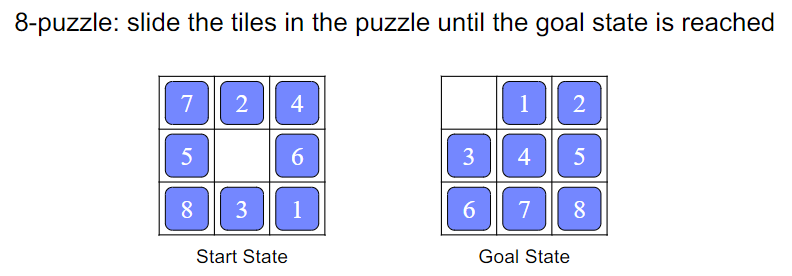
A relaxed problem is a simplification of your initial problem with lowered constraints. There can be multiple relaxed problems which can all give different heuristics.

For example, using the 8-puzzle above, we could allow tiles to be picked up and placed anywhere on the grid ($h_1=$ number of misplaced tiles) -> $h_1=8$.

Alternatively, we could allow tiles to be overlayed on top of each other when being moved ($h_2$ = the sum of Manhattan distances of tiles from goals) -> $h_2=18$.

These simplified problems will give us an underestimate (therefore admissible) heuristic. The closer a heuristic estimate is to the true cost, the more effective the A* search.

Sub-Problems

Sub-problems involve breaking down a larger problem, finding the exact cost of solving a smaller sub-problem, and then caching the cost.

For example, using the 8-puzzle above, the sub-problem could be trying to only move 1, 2, 3, 4 to the goal positions.

Assessing Heuristics

Quality of a heuristic can be expressed as its effective branching factor $b^{\ast }$, which can be determined empirically. The closer $b^{\ast }$ is to $1$, the better the heuristic.

Assuming A* visits $N$ nodes and finds solution at depth $d$:
$N=1+b^{\ast }+(b^{\ast }{)}^2+\dots +(b^{\ast }{)}^d=\frac{(b^{\ast }{)}^{d+1}-1}{b^{\ast }-1}$

We can approximate the effective branching factor for larger values of $b^{\ast }$:
$b^{\ast }\approx N^{1/d}$

---

CITS3011 - Lecture 4