CITS3011 - Lecture 4

← Back to Home

CITS3011 - Lecture 3
Game Playing - Slides

Game Playing Agents

Real world problems are rarely complete or deterministic (e.g. sensor limits, intractability, randomness). Games give a controlled, well-defined testbed for these issues, and introduce adversarial agents.

Adversarial Agents

Most games involve different parties making turn-based decisions. An agents need to take into consideration how other player’s might act, and the consequences of those actions.

Formulating a game:

Function	Meaning
$S_0$	Initial state at game start.
ToMove(s)	The player whose turn it is to move in state $s$.
Actions(s)	Set of legal moves in state $s$.
Result(s,a)	Transition model, defining state $s$ resulting from taking an action.
IsTerminal(s)	Terminal test, true when game is over.
Utility(s, p)	Final numeric value to player $p$ at terminal states. Used to pick best choice.
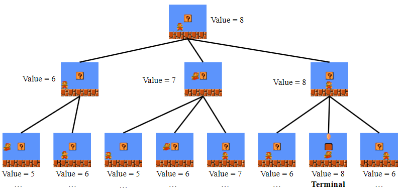
Starting from an initial state, we can generate a set of actions downward to create a game tree.

Minimax Algorithm

The minimax algorithm is a decision-making algorithm used to determine the optimal move for an agent in a two-player, turn-based, perfect-information and zero-sum game (e.g. Chess, Checkers or Tic-Tac-Toe).

A zero-sum game is a situation where one person's gain is exactly balanced by another person's loss.

The algorithm simulates the game by defining two players, named MAX and MIN. We use a utility/value to describe the game position. The utility function is positive if the state is good for MAX and negative if the state is good for MIN.

The game tree is generated top-down. Then, the utility function is applied to the leaves, giving us a score for each final board state. These scores are then passed back up the tree (recursion), to give a value for every state.

A ply means to move by one player, bringing us one level deeper in the tree.

As minimax generates the entire tree of possibilities, it is both complete and optimal (against an optimal opponent). It is usually implemented using DFS, giving us a lower space complexity.

Time Complexity	Space Complexity
$O(b^m)$	$O(bm)$

Example minimax implementation:

function minimax(position, depth, maximisingPlayer)
  if depth == 0 or game over in position
      return static evaluation of position
 
  if maximisingPlayer
    maxEval = -infinity
    for each child of position
      eval = minimax(child, depth - 1, false)
      maxEval = max(maxEval, eval)
    return maxEval
 
  else
    minEval = +infinity
    for each child of position
      eval = minimax(child, depth - 1, true)
      minEval = min(minEval, eval)
    return minEval

Cutting Off Search & Evaluation Functions

For a complex game, standard minimax is not suitable as expanding to the terminal states is infeasible, due to the amount of possible paths. Thus, we usually use either a cut-off test (e.g. a depth limit) or an evaluation function (i.e. a heuristic to determine state desirability).

Implementing a depth limit is useful for simpler games. Iterative-deepening (an anytime algorithm) can be used to adjust search under time constraints. But if we cut-off the depth, how do we compute the value of the state (since state value is computed bottom-up)?

This is where we can apply a evaluation function to the states at the cut-off depth in order to judge how good of a position the state is in.

For example, we could use a linear weighted sum of relevant features to evaluate the state of a chess board. Points are given for pieces, plus positional (e.g. centre control) and dynamic considerations (e.g. threats).

A good evaluation function should agree with the utility function at terminal states, reflect probability of winning and be fast to compute. The effectiveness of the player depends critically on the effectiveness of its evaluation function.

Alpha-Beta Pruning

Alpha-beta pruning is an optimisation technique for the minimax algorithm that dramatically speeds up the search process. It cuts-off branches in the game tree that don’t need to be evaluated because a previously, examined branch already guarantees a better outcome.

In the scenario below, the black and white dots represent the MIN and MAX players respectively. We know that the MIN player (black), will make the choice that will likely end with the smallest score.

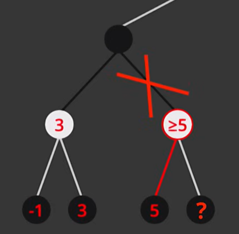
After examining the bottom two nodes, we get $(-1,3)$ as the two outcomes. White, the MAX player will choose the rightward option, meaning we can set that node’s score to 3. For the other white node, we find that one of its children would result in a score of 5.

Given this information, we know that the (right) white node must be $\ge 5$ as if the ? node is $\le 5$, it would not be chosen due to it not benefiting the white player. But since the parent node is $\ge 5$, the black player will not choose this path, as the left path is always better. So we do not need to examine the ? node and can ‘prune’ the rightmost child branch.

Building upon our minimax implementation, but with alpha-beta pruning:

function minimax(pos, d, alpha, beta, maximisingPlayer)
  if d == 0 or game over in pos
      return static evaluation of pos
 
  if maximisingPlayer
    maxEval = -infinity
    for each child of pos
      eval = minimax(child, d - 1, alpha, beta, false)
      maxEval = max(maxEval, eval)
      alpha = max(alpha, eva1)
      if beta <= alpha
	    break
    return maxEval
 
  else
    minEval = +infinity
    for each child of pos
      eval = minimax(child, d - 1, alpha, betam true)
      minEval = min(minEval, eval)
      beta = min(beta, eva1)
      if beta <= alpha
	    break
    return minEval

Whether pruning occurs or not depends on the ordering of moves. We want to test expected good moves first, as that will lead to more prunes. Pruning does not affect the final result, it just reduces computations.

---

CITS3011 - Lecture 5