CITS3011 - Lecture 6

← Back to Home

CITS3011 - Lecture 5
Probabilistic Reasoning - Slides

Product Rule

Product rule states that the joint probability of two events occurring together is found by product of the probability of the first event and the conditional probability of the second event occurring given that the first has already happened.
$P(x)\times P(y\mid x)=P(x,y)$

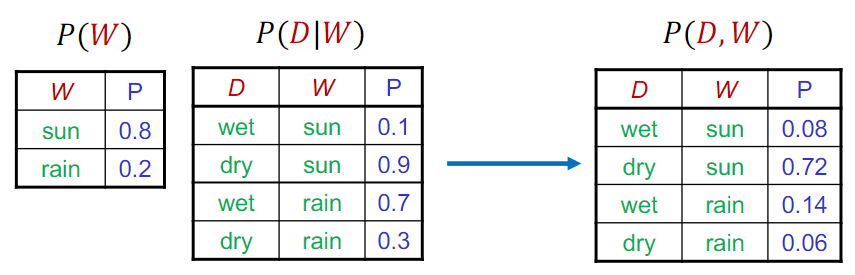
Product rule can be applied to probability distribution tables:

---

Chain Rule

Chain rule (also known as general product rule) allows you to calculate the joint probability of any number of events by breaking it down into a sequence of conditional probabilities.

Chain rule for 3 variables:
$P(x_1,x_2,x_3)=P(x_1)\cdot P(x_2\mid x_1)\cdot P(x_3\mid x_1,x_2)$

Chain rule for $i$ variables:
$P(x_1,x_2,\dots ,x_n)={\prod }_{i=1}^{n}P(x_i\mid x_1,\dots ,x_{i-1})$

---

Bayes’ Rule

Bayes’ rule (also known as Bayes’ theorem) is a mathematical formula that lets you update the probability of an event new evidence/data is acquired.
$P(A\mid B)=\frac{P(B\mid A)\times P(A)}{P(B)}$

Term	Name	Description
$P(A\mid B)$	Posterior	Updated probability of $A$, after new evidence $B$.
$P(A)$	Prior	Initial baseline probability of $A$.
$P(B\mid A)$	Likelihood	Chance of $B$ if hypothesis $A$ were actually true.
$P(B)$	Marginal	Total chance of $B$ under any and all circumstances.
Bayes’ theorem is helpful as it allows us to build one conditional from its reverse. Sometimes one conditional is difficult to find, but the other is simple. A common real life use-case is in medical diagnosis, where we must account for false-positives.

---

Independence

Independence means that the probability of two events are unrelated to one another. The outcome of one event has no impact on the probability of the other.
$P(A\mid B)=P(A)$

Conditional Independence

Two events $A$ and $B$ are conditionally independent given a third event $C$ if, once you know whether $C$ happened, knowing $A$ gives you no new information about $B$.

This is because the variable $C$ is the hidden link that causes both $A$ and $B$, and without examining it directly, it can make $A$ and $B$ seem highly dependent on each other.

$P(A\mid B,C)=P(A\mid C)$

---

Naïve Bayes Classifier

The Naïve Bayes classifier is a fast, probabilistic machine learning algorithm based on Bayes’ rule. It is called ‘naïve’ because it makes an unrealistic assumption that all input features are completely independent of each other.

Classifiers

A classifier is a machine learning algorithm used to assign data points into predefined categories or “classes”. For example, a classifier can read an email and decide if it belongs in the “Spam” or “Inbox” class.

The classifier is incredibly fast and highly scalable as it only needs to calculate individual feature probabilities independently, instead of computing complex multidimensional interactions.

For example, if you feed the algorithm a picture of a red, round fruit with a stem, it calculates the probability that it’s an apple by looking at “red”, “round”, and “stem” entirely separately. It completely ignores the fact that these features usually correlate with each other in real life.

Despite the drastic assumption of the model, it is usually good enough at used as a quick baseline to determine if a more complex algorithm is actually worth the extra computing.

---

Bayesian Network

A Bayesian network is an advanced probabilistic model that maps out the exact cause and effect relationship between different variables.

Full joint distribution tables ($d^n$) are ineffective for a large number of variables; for just 20 Boolean variables ($d=2)$, you would need $2^{20}$ rows. The compact nature of a Bayesian network ($n\times d^{(k+1)}$) is preferred; $k$ is max # of parents and is always much smaller than $n$.

In a Bayesian network, the nodes represent variables and the edges between them represent interactions. These interactions usually represent conditional independence between variables.

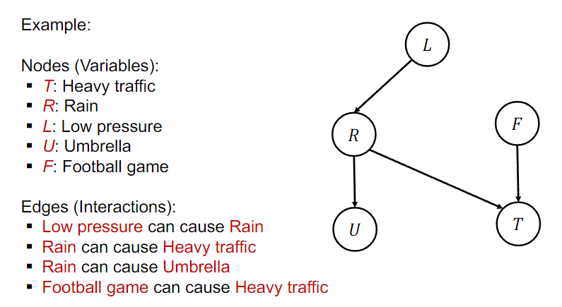
Nodes can represent total or dependent probability for a parameter depending on whether it has edges running into it:

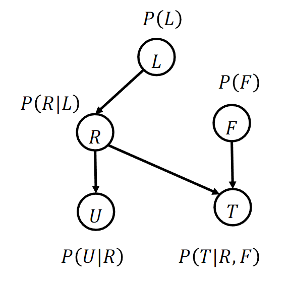
At each node, we give the conditional probability table:
$P(\text{node}\mid \text{its parents})$

Computing a Full Joint Probability

To find the exact probability of a complete scenario across all variables simultaneously, we can factorise the joint distribution:

$P(x_1,\cdots ,x_n)={\prod }_{i=1}^{n}P(x_i\mid \text{parents}(x_i))$
A node is completely independent of its ancestors once you know the status of its immediate parents.

In order to determine edges for a Bayesian network, the general rule is the a node is conditionally independent of its non-descendants, given its parents.

D-Separation

D-Separation is a criterion used to determine whether two sets of variables in a Bayesian network are conditionally independent of each other, given a third set of observed variables (evidence).

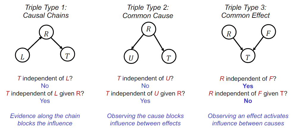
If all paths between two variables $X$ and $Y$ are blocked by evidence set $Z$, then $X$ and $Y$ are D-separated:
$X\perp \perp Y\mid Z$

Active / Inactive Triples

An active triple is a path of three connected nodes where information flows freely. Observing a change in the first variable affects our belief about the third variable.

Conversely, an inactive triple is a path where the flow of information is blocked because an intermediate node has been observed and D-separates the other two nodes, or because a common effect remains unobserved, keeping its parent variables entirely disconnected.

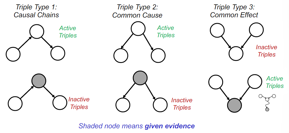
In the examples above, the shaded node is $Z$, where we have direct data about its state. For casual chains and common cause, the unshaded nodes are D-separated by $Z$. The opposite is true for common effect, where $Z$ connects the two parent nodes.

With $Z$ present, they provide no additional information about one another and are thus conditionally independent.

---

CITS3011 - Lecture 7